6. Bertrand-paradox

• The Bertrand paradox (in fact not a paradox) is an example of a seemingly simple probability variable can be achieved in a variety of ways if its definition is not clear enough. The Bertrand paradox goes as follows: Consider an equilateral triangle inscribed in a circle. Suppose a chord of the circle is chosen at random. What is the probability that the chord is shorter than a side of the triangle? (from Wikipedia) Depending on the arguments, there are three possible valid answers:
  1. The first assumption is to choose a random direction (by symmetry this can be any, so even the horizontal one) and the chord is selected from the perpendicular ones, randomly choosing a point on the horizontal diameter of the circle.
  2. The second assumption is to choose one point of the circumference of the circle and the other endpoint of the string is an other randomly chosen point.
  3. The third assumption is to choose a point from inside the circle (evenly distributed) and through it draw a string perpendicular to the line joining this point to center.
• All three assumptions and solutions (a bit differently formulated) with illustrative and enjoyable animations can be seen in a page of MIT. (Before reading this solution, you should think a little bit on it!)
• Let the radius of the circle is 1, so its diameter is 2, and mark the string length in an experiment by \(X\), i.e. \(X\) is a probability variable with values between 0 and 2. The task will be to write a code, which simulates all three models \(N\) times, records the lengths, and construct the three experimental cumulative distribution functions. The experimental cumulative distribution function at \(x\) will say that how much is the relative frequency of the \(\{X < x\}\) event. This is a step function. 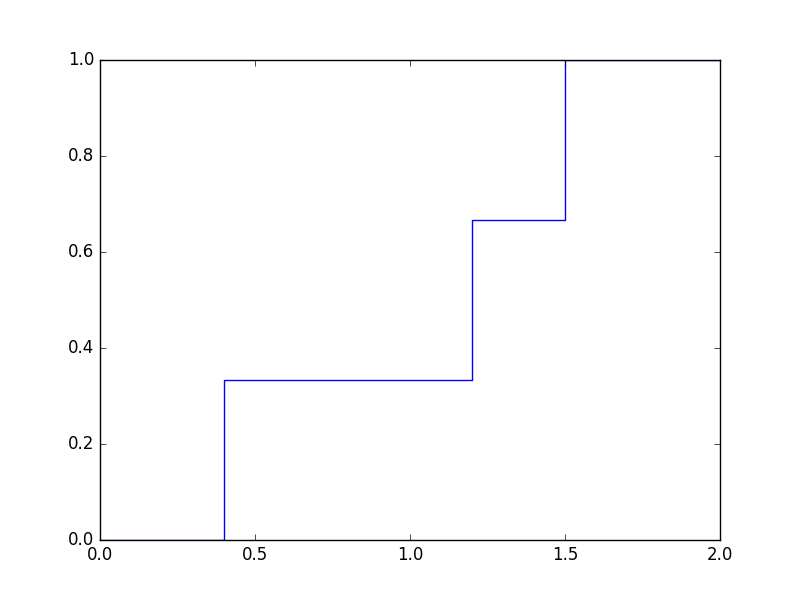(The cumulative distribution function is defined by \(F_X(x)=P(\{X < x\})\).) For example, if you make three experiments, and the string lengths are 1.5, 0.4 and 1.2, then the graph of the empirimental cumulative distribution function looks like this (the graph made by the step function of the matplotlib.pyplot library; do not worry about the vertical lines in the graph, and consider the function at these places continuous from the left):
  
• The three models have to be implemented in the file available here. The output should be the graphs of the three experimental cumulative distribution functions in a single picture. The common domain is the interval [0,2]. Obviously all three functions are increasing, the value at 0 is 0, at 2 is 1, and the value at \(\sqrt{3} \approx 1.732\) is approximately \(1/2\), \(2/3\) or \(3/4\) depending on the model.
• Implementation:
  • First model: choose a random number \(r\) from the interval \([-1,1]\), and calculate the length of the chord perpendicular to the horizontal line at \((r,0)\) (use the functions acos and sin from the modul math.
  • Second model: let the first point be \((1,0)\), and the second be a random point from the line of the circle, that is the point \( \cos \alpha, \sin \alpha\), where \(\alpha \) is a random number from the interval \([0, 2 \pi )\).
  • Third model: choose an arbitrary pont from the square \([-1,1] \times [-1,1] \) (that is choose two random numbers from the interval \( [-1,1]\), and make a pair from them), and check if it is inside the circle. If not, choose an other one, and so on. The length of the chord can be calculated similarly to the first model.
  • Drawing the experimental cumulative distribution functions: after simulating \(N \) experiments, sort the numbers with the sort() method. Write a \(0\) at the beginning of the list and a \(2\) at the end. This list gives the points on the horizontal axis. Above these points the step function "jumps." At each point the value of the function is increasing by \( 1/N \). If the length of the shortest cord is \(r\), then the value of the function over \([0,r]\) is \(0\), so the list of function values is \([0,0,1/N,2/N,\dots, 1]\). 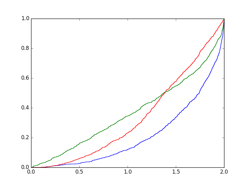For drawing the file uses the function matplotlib.pyplot.step(x,y) where \(x\) and \(y\) are the two previously constructed lists. A possible result for \(N = 1000\) is shown in the following figure:
    
• To file to be uploaded has to be called Bertrand.py. After completing this program, do experiments with different values for \(N\). Finally make your program runable from terminal. For example in the case \(N=100\) execute the program with

    python3 Bertrand.py 100
  

• The aim of this task is to help understanding the continuous random variable, its cumulative distribution function and the approximation of it from experiments. There is no essential new topics in Python programming.